HOW TO DECLUTTER YOUR SPREADSHEETS BY HIDING ZERO VALUES
Are your spreadsheets filled with unnecessary zero’s, cluttering your information and making it hard to identify significant results?
Undertaking data analysis in Excel quite often results in your formulas returning zero’s simply because they point to cells that do not contain any data. I know I come across this ALL the time as I attempt to make my spreadsheets as flexible as possible.
Using our D.A.R.E. Methodology, I break spreadsheets down into a Data area and an Analysis area. In the Analysis area, I’ll typically copy formulas over a large area so that when I add information into the Data area, I minimise my workload by not having to adjust/extend formula ranges, etc. Sorry if that sounds confusing. Don’t worry too much about it as that is not the point of this article. What you need to take from it is that when you have a LOT of formulas in your spreadsheets, often you’ll find a LOT of zero’s in your results which can potentially hide significant results.
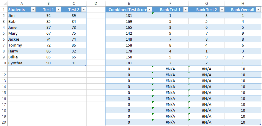
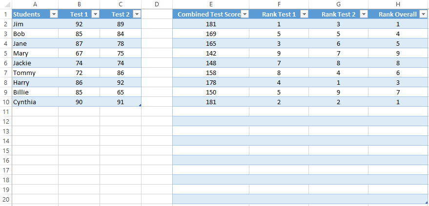
The example below shows some data entered into the range A2 to C10. I have an Analysis area setup with formulas in cells E2 through to H20. In this example, the number of students in Column A can vary up to a maximum of 20 pupils. To minimise my future workload, I have entered formulas in columns E to H right down to row 20, but as you can see this means our Results table has unnecessary zeros appearing where they don’t need to be.
Two ways to hide zeros in your spreadsheets
So how do we hide these unnecessary zeros from our spreadsheets?? Fortunately, there are two quick alternatives to address this issue.
A quick note before we go through these methods. The 2 methods described below only affect the appearance of what is displayed in the cells. They do nothing to the actual underlying values stored in these cells – hence the zeros are still there, we are just getting Excel to apply some formatting tricks to make them appear as though they have disappeared.
1. Hide ALL zero values
One way we can hide all zero values in our spreadsheets is by modifying a setting in Excel itself.
Navigate to File > Options > Advanced. Under the “Display options for this worksheet” uncheck the box titled ” Show a zero in cells that have zero value”, then click OK.

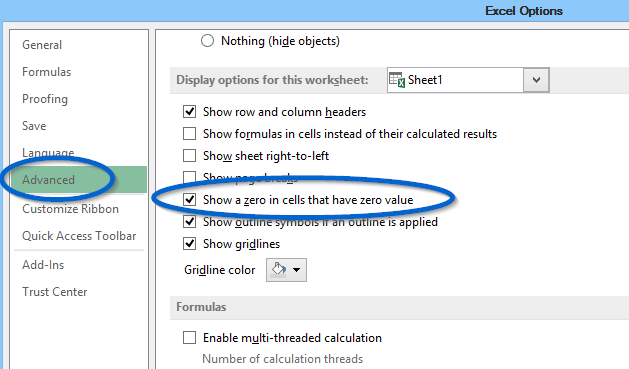
This option, while it being quick and simple, has a huge downside in that it will hide ALL zeros throughout your entire spreadsheet. It will not distinguish between ‘significant’ or ‘insignificant’ zeroes. In other words, if you manually input a zero into a cell, or if zero is the correct output of a formula, these values will be hidden alongside all the other insignificant zeroes.
I would file this option under “Just because something can be done, doesn’t necessarily mean it should be!!”
2. Custom Number Formatting
While slightly more complicated, a better method for hiding ‘insignificant’ zeroes is to use custom number formatting across your range of cells. Custom number formatting simply applies different formats to your cells depending on the criteria you enter.
To apply custom formatting to our cells in Column E for example:
- Left click and drag cells E2 to E20
- Right-click on one of the selected cells and select Format Cells
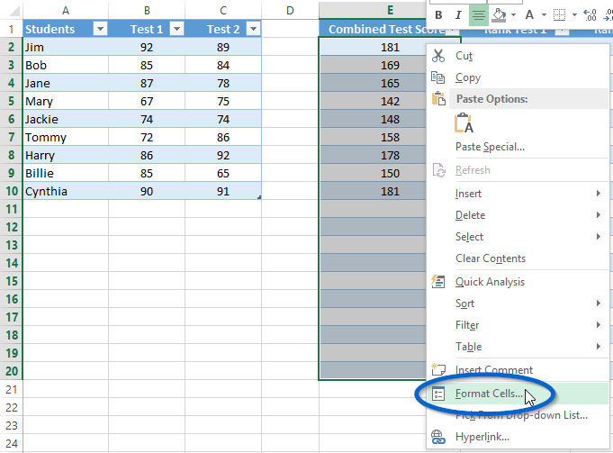
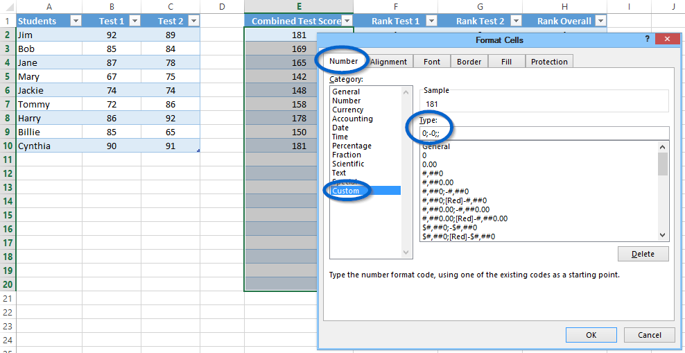
- Under the Number tab, click Custom
- In the textbox that appears below the word “Type:” delete the word “General”
- Now in the same textbox type 0;-0;;@ and click OK.
Custom Number Formats
Excel lets you change the format of the ways it displays data in a cell. For example, you can specify the number of digits to the right of a decimal point, or you can add a comma separator when displaying large numbers. You can access and modify the majority of these settings in the Format Cells dialog box.
To apply a custom format to a cell, it is very important to understand how cell formats are seen by Excel. Excel sees a cells format as having four individual sections.
These are:
- positive numbers;
- negative numbers;
- zeros; and
- text.
Each of these Sections are separated by a semi-colon (;). These code sections define the format for <POSITIVE numbers>;<NEGATIVE numbers>;<ZERO’s>;<and TEXT> in that order.
So in our example above where we entered 0;-0;;@ we are telling Excel to display positive numbers; display negative numbers; do not display zero’s; and display text
There you have it. Apply either one of the two methods above and those unwanted zeroes will be a thing of the past.
Download
Click the following link to download a PDF transcript of this tip.
We also have available for you to download a copy of the spreadsheet we used in this article. Feel free to also download a copy of it so you can explore this tip even further.
![]() PDF Transcript – Declutter your Spreadsheets by Hiding Zero Values.
PDF Transcript – Declutter your Spreadsheets by Hiding Zero Values.
![]() Excel File – Declutter your Spreadsheets by Hiding Zero Values.
Excel File – Declutter your Spreadsheets by Hiding Zero Values.
Continue the Discussion
So do you try and hide zero’s in your spreadsheets? If so, how do you do it? Do you use either of the methods described above or do you use another method? Continue the discussion and add your thoughts in the comments section at the bottom of this article.
Please Share
If you liked this article or know someone who could benefit from this information, please feel free to share it with your friends and colleagues and spread the word on Facebook, Twitter and/or Linkedin.
