Excel Kick-Starter eCourse.

This Kick-Starter eCourse will provide you with down-to-earth, practical information to get you kick-started creating your own spreadsheets; adding and modifying data and then save and close your spreadsheet for later use. You will also cover how to save time by using formulas; how to format your data to make it look professional; as well as how to add a chart to highlight trends. Last but not least, we will also cover some time saving tricks by introducing you to keyboard shortcuts.
Throughout this eCourse, the steps and screenshots shown are based on Microsoft Excel 2013. If you are using a different version of Excel, the basic principles will be the same, however, you may find that some of the steps and screens we reference may look and act a little different.
As with most things Microsoft has created or developed, there are usually many ways to undertake the same tasks in Excel. We do not discuss all the different ways to undertake all the tasks in this article, but rather explain the ones we personally use and recommend or the ones that make the most sense in the particular situation we are discussing.
With that out of the way, let’s dive in and start exploring Microsoft Excel.
So what are we covering in this eCourse?
To help you work through this eCourse and so you can see how this information can be applied to a real-life situation, we are going to be using a case-study. The information we learn will be applied throughout the case-study so you can see how you might apply it in your particular circumstance.
Case Study:
Helen has just started work at a small to medium enterprise (SME) and has been given the task of producing a quarterly sales report, identifying sales trends for each of their regional offices, for the company’s CEO.
Helen being brand new to the role, has little to no previous experience using Microsoft Excel and has to design the report from scratch.
So how does Helen undertake this task??
The 6 CORE components that Helen is going to use to, not only simply get the job done but impress her new boss are:
Core Component:
1. Understanding the Main Elements of Excel
Before Helen can start developing her spreadsheet, she first had to take just a little time to get familiar with Microsoft Excel. She was aware that that Excel is a spreadsheet program. But what is that? A spreadsheet allows Helen to enter data into it so that it can be organised, manipulated, calculations performed and undertake some analysis. It is an extremely powerful tool that she was about to learn how to use.
With it being such a powerful tool, it contains many things that for day-to-day applications Helen will typically never use (most Excel users usually only scratch the surface with what they can do using this tool).
Not wanting to waste her valuable time, this eCourse only covers the core 6 components that are needed to get up and running and productive in as short a time as possible. It leaves the more advanced features and functionality to be learnt another time.
Within this first section, Helen will learn:
![]()
- What are Rows, Columns and Cells?
- What is the Ribbon?
- Workbooks and Worksheets
- How to create/open a Workbook
- How to Save a Workbook
- How to Print a Worksheet within a Workbook
- How to Close a Workbook
What are Rows, Columns and Cells?
When Helen first opened Excel on her computer, she saw the main screen which looked something like the following image. It at first looked quite intimidating to her. But, she feared not, as she knew this eCourse would explain what she needed to know in a straight-forward manner so she could get used to the way everything works.
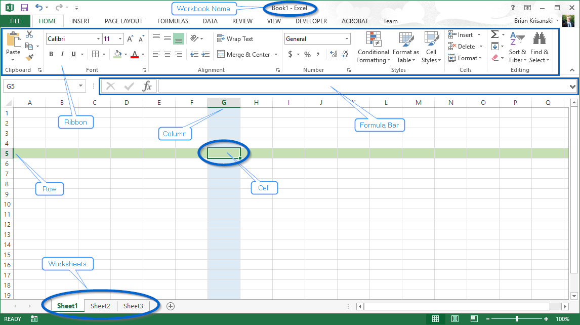
Excel – main screen components.
One of the first things Helen noticed was that the main working area looked a lot like an accounting book ledger. It consisted of a grid style interface that is made up of rows and columns. Each individual row is identified by a number – 1, 2, 3, 4, etc and a column by a letter – A, B, C, D, etc.
The intersection of each row and column is called a cell. Cells within Excel are referred to by their corresponding row and column i.e A1. In the above image, the highlighted cell, is at the intersection of column G and row 5, and can be referred to as the cell at position G5. Helen found this easy to understand as it is much like one of her beloved childhood game’s “Battleship”.
![]()
What is the Ribbon?
Looking just above the “grid” Helen saw the Ribbon. It runs right across the top of Excel.
The Ribbon was designed to be more intuitive than the old drop-down style menus in other software programs.

Excel – Ribbon.
Helen noticed that the first tab that is visible is the Home tab. She realised that this tab contains most of the basic functions that she would be using on a day-to-day basis. The other Tabs she saw were: Insert, Page Layout, Formulas, Data, Review and View.
The tabs you see in the Ribbon contextually change. Emphasis is placed on the tools and options that are relevant to the task you are undertaking at the time. For example, if you are creating a chart, a “Chart Tools” menu option becomes available to you to provide you with all the tools and functions that you need to create and format your charts.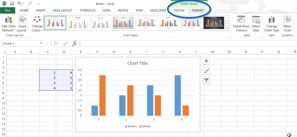
Excel – Ribbon Chart Menu.
In the image above, towards the right-hand side of the menu, there is also a Developer tab. This Tab may or may not be showing for you. By default, Excel does not show this tab. If you don’t do any programming or writing macros etc, then you don’t have to worry about it. If you are interested in how to get the Developers Tab to show in the Ribbon – this articles explains all you need to know.)
Workbooks and Worksheets
Simply put, a workbook is just another word for your Excel spreadsheet. Excel automatically creates a blank workbook when you start it up.
Now worksheets are the collection of cells where you enter, organise and manipulate your data. By default, each Excel workbook contains three worksheets.
Confused?? Don’t worry Helen was as well. that was until we got her to think of both of these like – think of a workbook being like a manilla folder and inside that folder you can have one (or more) sheets of information (the worksheets). Each sheet of information is a separate worksheet inside your workbook.

Workbook containing 3 worksheets
How to Create/Open a Workbook
The first step for Helen to start working on her sales report is to create a new workbook for her to store all her data.
Create a new Excel workbook
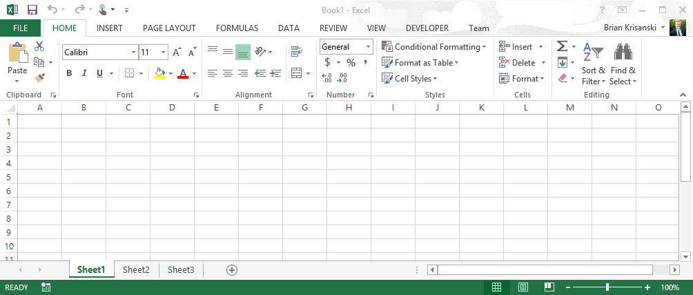
Helen’s newly created Excel workbook with three blank worksheets.
Open an existing Excel Workbook
Helen will not always be creating new Excel workbooks every time she uses Excel. In most cases, she’ll be wanting to open already existing workbooks to modify or update them.
To open an existing workbook:
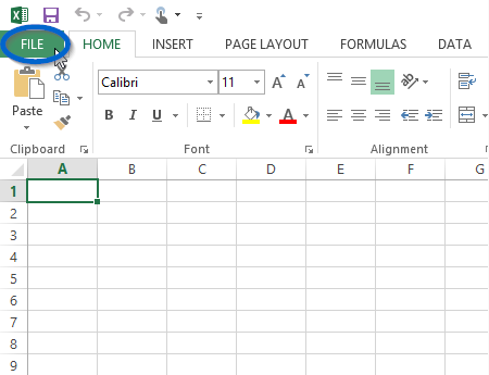
Click the “File” tab in the Excel Menu
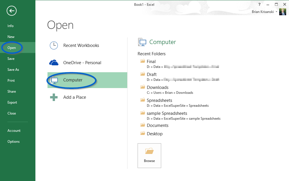
Microsoft Excel Open dialogue window
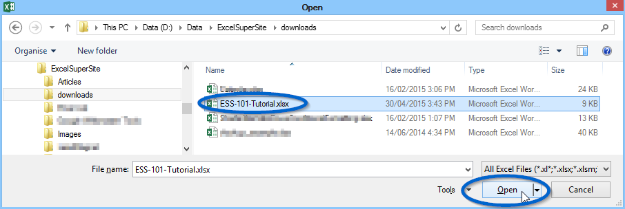
Open workbook dialogue box

Open an existing workbook
How to Save a Workbook
There are not too many things worse that can happen to an Excel user than spending countless hours working on a spreadsheet and then having an issue with your computer that causes Excel to unexpectedly close or having a power outage and your computer shuts down before you have had the chance to save your hard work.
This can be VERY, VERY, VERY frustrating. (Unfortunately speaking from past experience…)
One thing Helen learnt very early on was to make sure she always saved her work and to make sure she saved it often.
Excel has some excellent Autosave and file recovery features built in to help you retrieve your work if the unfortunate happens. We will not go into these features here, but if you have ever thought you have lost your work, you “may” be able to retrieve it (or most of it) by using Excel’s Autosave or file recovery tools. However, best not to rely on these tools and make sure you frequently save your own work.
To save a workbook
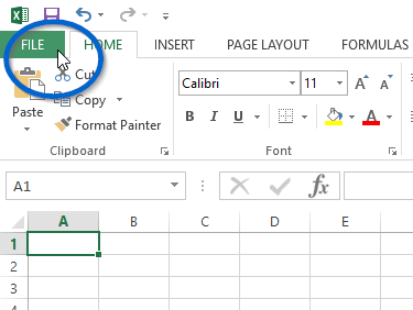
Click the File Tab
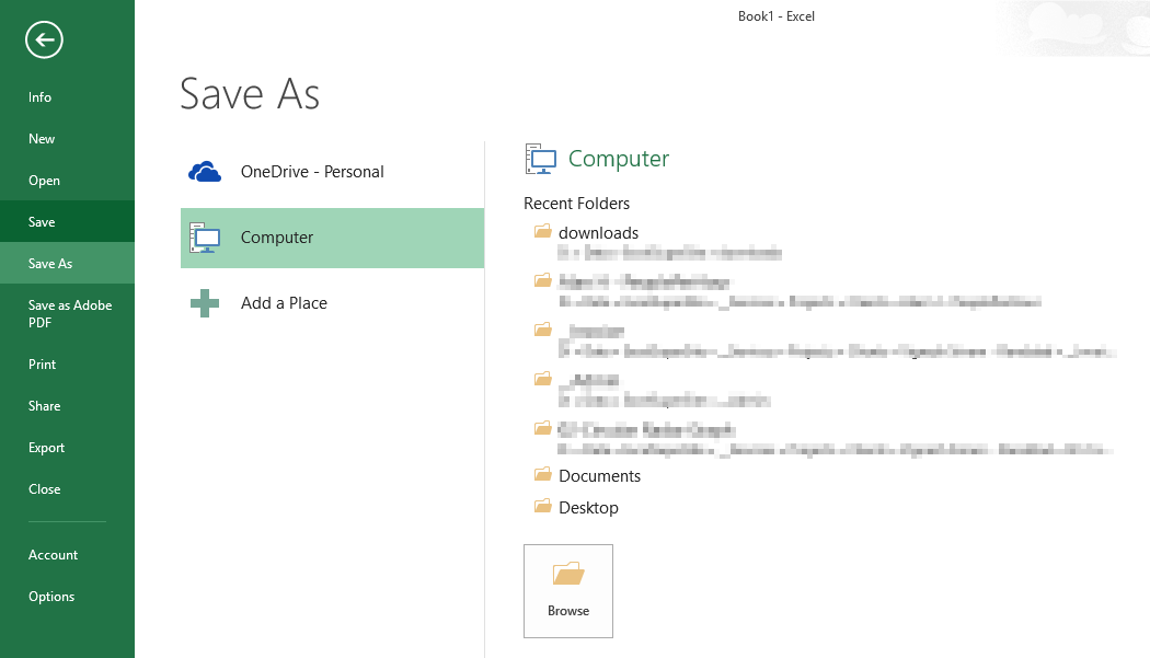
Select where you want to save your spreadsheet
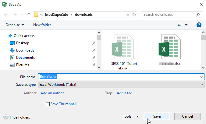
Click Save to save your spreadsheet
You’ll notice under Save As (in the image above) you have three options: SkyDrive, Computer, and Add a Place. The first option is SkyDrive. If you select this option you will be saving you spreadsheet “in the cloud” on servers operated and controlled by Microsoft. This is very useful if you want to work on your Excel documents from multiple locations or on different devices. For example, you may be working on a spreadsheet in your office, saving it to SkyDrive means you’ll also be able to open it and continue to work on it when you get home.
How to Print a Worksheet in a Workbook
Quite often, after you have finished working on a spreadsheet you’ll want to print it out. In this section, we’ll go over how Helen can print her worksheet and how she is able to modify a few important print settings.
To print your worksheet

Click File then Print

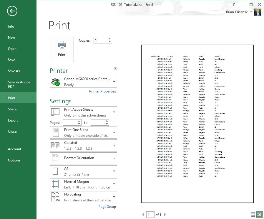
Print Preview
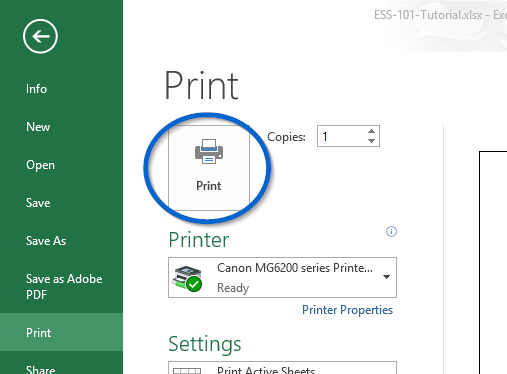
Click the Print button to print your spreadsheet
When printing her first worksheet, Helen noticed that there are a number of different settings she could adjust.
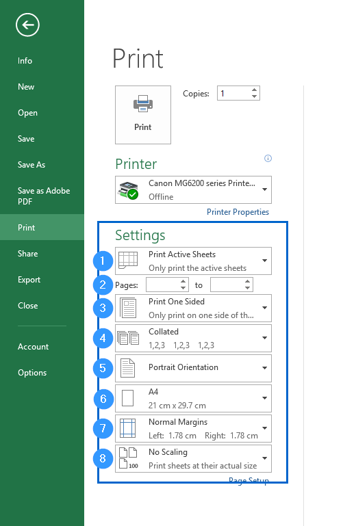 Print Settings
How to Close a Workbook
There are multiple ways in which you can close a workbook.
To close a workbook

Click the File Tab
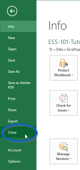
Close
Alternatively, a workbook can be closed by clicking the Close Button (cross) in the top right hand corner of the Excel window.
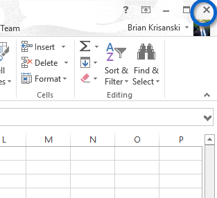
Click the Close Button to close the workbook
If you are trying to close your spreadsheet and it has not been saved, Excel will prompt you to save your workbook before it closes.

Save before closing dialog box
Action Steps
Core Component:
2. Entering and Editing information in a Spreadsheet.
Now that Helen is familiar with the Excel main screen and knows how to create, open and save an Excel Workbook, she is all set to start creating her spreadsheet that she is going to use to create the Quarterly Sales Report.
The next steps she needs to cover is how does she enter her data and make any corrections should she make a mistake.
- Entering data into a worksheet
- Editing data in my workbook
- Removing data from my workbook
- What if I make a mistake?
Entering data into a worksheet
To enter data into her Excel workbook, it is very simply a matter of Helen selecting the relevant cell on her worksheet, by left clicking it with her mouse and then simply started typing out her data. To move from one cell to the next, Helen needs to press the enter key on her keyboard or left click off onto another cell. Pressing the Enter key or clicking onto another cell adds your data into the Excel worksheet.
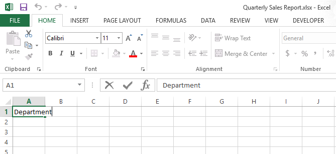
Type data then press ENTER to store your information
Excel has the ability to store a lot of data in many differing formats (numbers, text, dates, times, currency etc). If Helen were wanting to enter data in a different format, she simply needs to type the data as you would like to see it. Excel uses some smart background processes to try and “understand” the format of the data entered and how that data is intended to be displayed i.e. if Helen entered “$1,234.56” into a cell, Excel understands that she is are entering the number 1234.56 and that she wanted it displayed in a currency format.
While Excel generally does a good job of “understanding” the data being entered and how it should be formatted, it does not always get it right. But never fear, if it doesn’t get it right the first go, it can easily be changed so that it appears how it is intended. Formatting data will be covered further in Core Component: 4 Formatting Data to Make it Look Good.![]()
Editing data in my workbook
As Helen is not a robot and does not always correctly enter information into her worksheets all the time, there will be times (lots of them) when she will need to modify/update the information she has entered. Now she could just retype the contents of the cell all over again to re-enter the information, but I know Helen prefers to work smarter and not harder when it comes to these sorts of things (why do you think she is taking this course after all…). Rather than retype the entire cell contents, Helen wants to just change the number, text or part of a formula that needs to be modified.
To modify her data, first Helens must select the cell with her data (click the cell with her mouse) and then click into the formula bar (see image below). Once she has clicked into the formula bar, Helen can move back and forth through it and make the necessary changes. You can move in the formula bar with the arrow keys on your keyboard or by clicking the relevant spot with your mouse. After Helen has made the changes she wants, she simply presses enter key or left clicks onto another cell to add the changes to the spreadsheet.
Before forgetting, Helen makes sure she saves her work as she goes so that she does not lose any of it unexpectedly.
 Excel formula bar
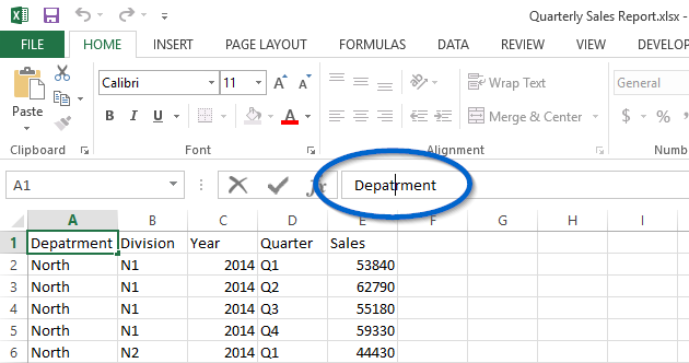
Cell A1 is active and the cursor is inside the formula bar
Another way to edit the data within a cell is by selecting the cell and then pressing the F2 key (function key at the top of your keyboard). This puts Excel into an edit mode which then allows Helen to make the modifications directly in the cell rather than via the formula bar.![]()
Removing data from my workbook
Removing data from Helens worksheets is also straight forward. If Helen only wanted to remove partial data from a single cell, all she needs to do is edit her data, taking out the text or numbers she no longer required, as described above. If Helen wants to remove the entire contents of a particular cell (or range of cells), she simply selects that cell (or range of cells) and then presses the delete key on her keyboard.![]()
What if I make a mistake
If you are in the process of making a modification to the information within a cell and then change your mind, provided you haven’t pressed enter or selected another cell, you can press the escape key and that will undo your changes and leave the information in the cell as it was.
If you have changed your mind after you have made a modification, Excel has an undo feature that allows you to undo your last actions. This feature can be indispensable. I’ve lost count of the numbers of times I have made mistakes, accidentally deleted something or changed my mind after I have made a change and have needed to revert back to the information in the cell before I “made” the change.
To undo a change, select the relevant cell, and then left click the Undo button to revert the last change made. If you wish to undo more than the last change made, click the small drop down arrow beside the undo button and click the changes to be undone.
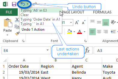
Undo button in Microsoft Excel
Action Steps
Core Component:
3. Using Formulas to Automate Calculations
Arguably, the most powerful feature of Excel is its ability to specify relationships between the data in its worksheets. With Helen having the ability to specify the relationships i.e. using formulas between her information, she is able to significantly enhance and improve the usefulness of her spreadsheets (and consequently her productivity as well).
Adding formulas to a worksheet allows Helen to turn her spreadsheets from static displays of data to useful tools being able to undertake calculations and highlight trends and results from her analysis.
Turning seemingly jumbled data into meaningful and useful information.
Excel Formula Structure
To begin with, let us break down the structure of a formula in Excel for Helen so she can see how she can start to use them.
Thankfully all formulas in Excel are generally constructed the same way. They all start with an equals sign (=) followed by one or more elements. The equals sign simply tells Excel that the data we are storing in a particular cell is a formula.
Each of the elements after the equals sign can be any or all of the following:
1. Constants
2. Operators
3. References
4. Functions
![]()
1. Constant
A constant is a value that is static and not the result of a calculation. For example, the numbers 1, 2, 3, 4 and 5 or even text like “ExcelSuperSite” are all examples of constants i.e. they do not change by themselves nor are they a result of a calculation.
A small but helpful tip:
Where possible, do not use constants in formulas. It is far better, from a spreadsheet design point of view, to use a cell reference that points to a particular cell that holds the constant data, rather than using the constant in the formula itself. That way you can easily change the value of the constant (if needed) without having to modify the formula itself.
2. Operators
Operators specify what type of operation (calculation) you want to perform on the elements in your formulas. There are four different types of operators that you can use:
b. Comparison
c. Text
d. Reference
| Arithmetic Operator | Description | Example Formula | Formula Result |
| + | Addition (plus) | = 3 + 2 | 5 |
| – | Subtraction (minus) | = 5 – 2 | 3 |
| * | Multiplication (times) | = 3 * 2 | 6 |
| / | Division | = 10 / 2 | 5 |
| % | percent | = 20% | 0.2 |
| ^ | exponential | = 3 ^ 2 | 9 |
| Comparison Operator | Description | Example Formula | Formula Result |
| = | Equals | = 3 = 2 | False |
| > | Greater than | = 5 > 2 | True |
| < | Less than | = 3 < 2 | False |
| >= | Greater than or equal to | = 10 >= 2 | True |
| <= | Less than or equal to | = 10 <= 2 | False |
| <> | Not equal to | = 3 <> 2 | True |
| Text Operator | Description | Example Formula | Formula Result |
| & | Concatenate (join) | = “Excel” & “Super” & “Site” | ExcelSuperSite |
| Reference Operator | Description | Example Formula |
| : | Range – references all cells between two references | =SUM(A1:A10) |
| , | Union – combines multiple range references | =SUM(A1:A10,C1:C10) |
| (space) | Intersection – references all cells common to the two references | =SUM(A10:D10 B5:B15) |
Just like when you calculate a normal maths problem, Excel follows basic maths principles when it undertakes calculations. Excel starts from the left and works to the right obeying maths precedence rules – B O M D A S (Brackets – Order – Multiplication – Division – Addition – Subtraction).
If you combine more than one operator into a single formula, you can change the order of evaluation by using parentheses to enclose the part of the formula to be calculated first.
As an example, the following formula results in 7 because Excel calculates multiplication before addition (obeying standard math precedence rules). The formula multiplies 2 by 3 and then adds 1 to the result.
However if we add parentheses to change the calculation order we can end up with a result of 9 instead. Excel adds 1 to 2 and then multiplies this result by 3 to give a total of 9.
3. References
References in formulas tell Excel where to look for data or information to use in your formula.
Excel makes reference to cells in a worksheet by using the column letter and row number of the particular cell. As an example, the cell reference C5 refers to the cell at the intersection of column C and row 5.
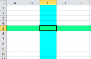
Cell Reference in Excel
References allow you to use the value from one cell in multiple formulas throughout your worksheets.
To try and explain this a little further, consider the following example:
Let’s say Helen needs to calculate 10% of the following list of numbers. Easy enough done. Simply enter a formula in each of the cells in column C as shown below.
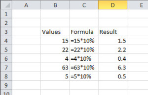
Simple formula in Excel using Constants
That was straight forward, so why would Helen need to use references instead of constants in her formulas? Consider the following extension to the above example. Instead of a list of 5 numbers, Helen now has a list of say 50 numbers and needs to calculate a range of percentages, say 5%, 10% and 15%.
Helen COULD do this exactly as done previously, but it involves a lot of unnecessary manual work. Don’t get us wrong, there is nothing wrong with hard work hard, but we also prefer to work smart.
Let’s get Excel to work for Helen rather than the other way round and Helen doing all the work.
Before we modify the formulas in column C, Helen first enters the percentage constant into cell C1 (she clicks cell C1 and enters 10%).
In cell C4 Helen types:
What this formula is saying is take the value of whatever is in cell B4 and then multiply that by the value of whatever is in cell C1.
Now copy this formula down to all the cells in column C.
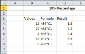
Formula using references in Excel
Entering the formula in this way, Helen can easily update the percentage constant in cell C1 to either 5%, 10% or 15% (or whatever value she likes), and she no longer needs to manually edit any of the formulas to get the results she is after. Similarly, all the values in column B could also be updated and we save ourselves a lot of work by having Excel do it all for us.
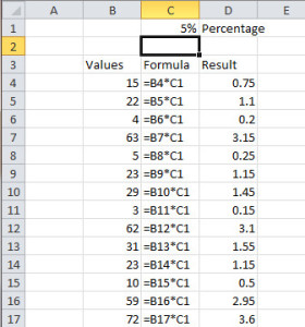
Formula references in Excel – 5%
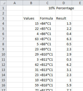
Formula references in Excel – 10%
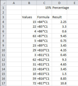
Formula references in Excel – 15%
| References | Type |
| Reference to the cell in column C and row 1 | C1 |
| Reference to the range of cells in column C and rows 1 through 10 | C1:C10 |
| Reference to the range of cells in columns C to E and rows 1 through 10 | C1:E10 |
4. Functions
Functions are predefined formulas in Excel that are available for use. A full listing of functions available to use can be found by clicking any cell in Excel and then pressing SHIFT & F3 (together) or by clicking the Insert Function button beside the Formula Bar (see the image below).
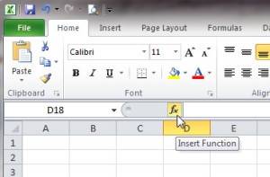
How to insert a function in Excel
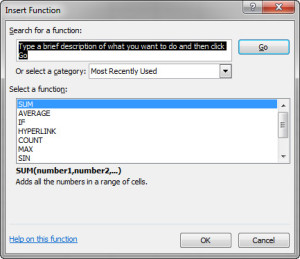
Insert Function dialog box
So how does all this information help Helen?
Quite simply, by specifying relationships (adding formulas) into her spreadsheet, Helen is able to significantly enhance the capabilities of it, allowing her to undertake analysis and highlight trends that are not easily visible by simply looking at the raw data.
Action Steps

Core Component:
4. Formatting Data to Make It Look Good
So now in Helen’s spreadsheet we have the raw data she requires to build her report. While the numbers are in the spreadsheet and they do show the information we need, they are not in a professional looking format and hence Helen needs to undertake a little more work to improve the look of her information before she can present it to her CEO.
Excel has a wide range of formatting options available to end users and it is relatively easy to turn a dull looking spreadsheet into something that really shines. An important point to remember when formatting data within a cell, is that you are only the modifying the appearance of the data. The underlying information does not change.
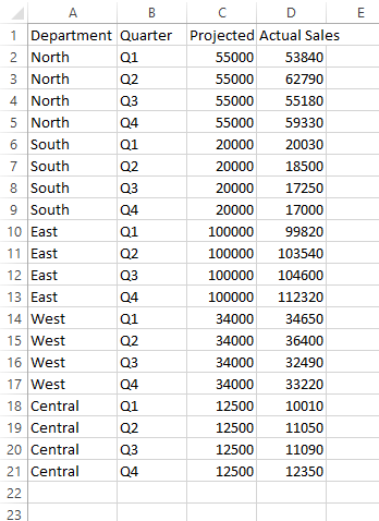
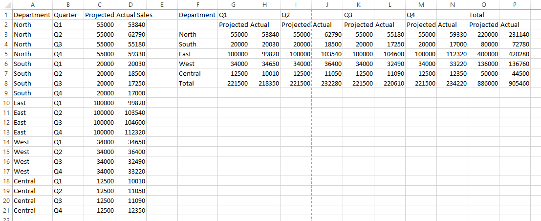
As an example, if Helen were to change the formatting of the data in cell D2 (53840), she can change the appearance of this value to something like $53,840.00 or 53,840 but the underlying data will always remain 53840.
When formatting a cell Helen can modify number formats (“53840”, “53,840”, “$53,840.00”, etc), but she can also make aesthetic changes as well (alignment, fonts, borders, colours etc).
Changing font, size and colour
To change the font/size/or colour of the data Helen has entered into her spreadsheet, she simply clicks on the cell (or range of cells) that she wants to format, then selects any of the different options in the Font panel in the Ribbon at the top of the page.
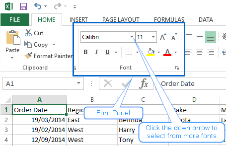
Font panel

The font in the Font panel above is currently set to Calibri. To see more fonts, click the black down arrow. One of the excellent things with Excel 2013 is that when you move your mouse over one of the fonts on the list, the text in your selected cell (A1 in this case) will change automatically showing you what the font style will look like. This is just a preview, though. When you have decided on the font you like, select that font with the left mouse button and Excel will apply it to your cell (or range of cells).
You can change the size of the font in the same way – just choose a new font size from the list of numbers in the drop down box beside the fonts.

The font colour can also be changed from here as well and similarly text effects like bold, italic or underlining.
To change the background colour of your cells, first highlight the cells you wish to modify. Then in the Font panel, click the Paint Bucket to apply the colour you see directly under it (yellow in our example). To change the colour that is applied, click the small down arrow just to the right of the Paint Bucket and select the colour of your choice.
Moving your mouse over any of the colours and the cells will change automatically showing you what the cells will look like. Similarly to the font selection, this is only a preview and the colour change does not get applied until you click it with the left mouse button.
If you don’t like any of the colours displayed, click on “More Colors” to see further colour selections.
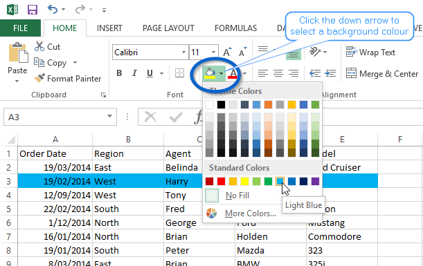
Change background colour
To change the colour of the text itself, click the down arrow just to the right of the letter A, which is just to the right of the Paint Bucket on the Font panel.

Select a colour just like you did for the background colour of a cell.
So as you can see, with just a few clicks of your mouse, Excel makes it very easy for you to change the look and feel of a spreadsheet.
Action Steps
- Bold all headings
- Center all text in columns G through P
- Format the figures in cells G3 to P8 as currency ($) with 0 (zero) decimal places showing
- Add a dark border right around the outside of the summary table
- Add a border between rows 2 and 3
- Add a border between rows 7 and 8 to distinguish the Totals figures
- Add a faint solid line between columns F and G
- Add a solid between columns N and O to distinguish the Totals figures
- Add a background colour to the headings (cells F1 to P2)
- Add a dashed line between columns H and I; J and K; L and M to distinguish the quarters

Core Component:
5. Create Charts to Highlight Trends
Helen, now has her summary table all ready to go, but to impress her CEO, she has decided to chart her results.
As the old saying goes “A picture is worth a thousand words” and this is none more so than when we are talking about Charts in Excel.
Charts are used to display numerical data in a graphical format, making it easier to show results and highlight trends. Excel supports many differing types of charts to display data in ways that are meaningful to your audience.
Create a basic chart
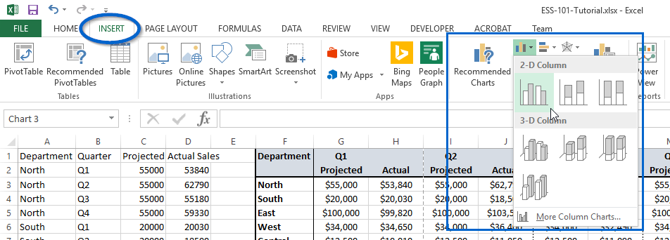
Insert a Clustered Column bar chart
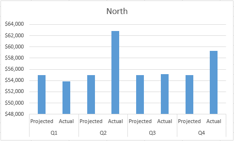
Clustered Column Bar Chart
Modifying the style of a chart
After you create a chart, you can instantly modify its look by adjusting its format.
If you don’t want to manually change chart elements or the formatting of your chart, you can try applying a predefined style to your chart.
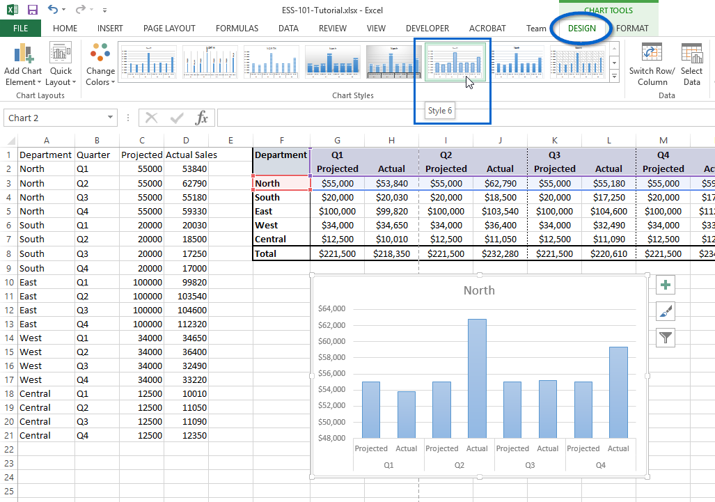
Applying a predefined Chart Style
Modify chart elements
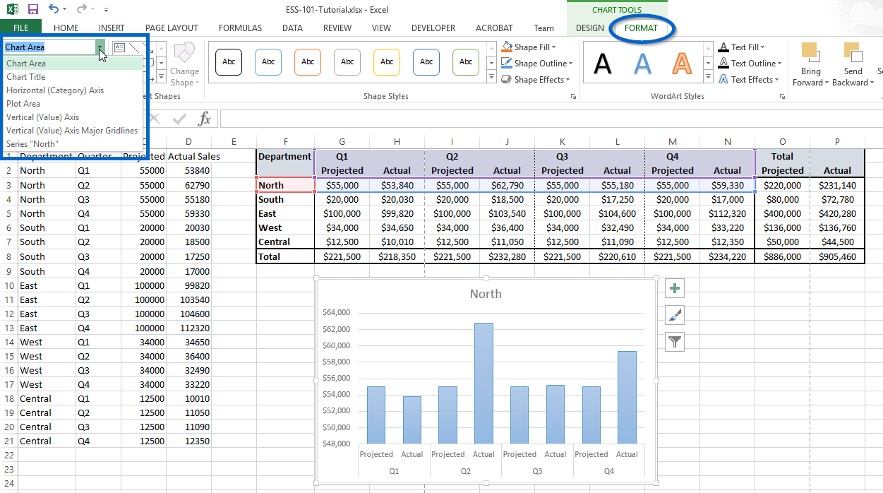
Format chart elements
Add Chart and Axis titles
To make a chart easier to understand, you can add chart titles and axis titles to display more information.
To add a chart title
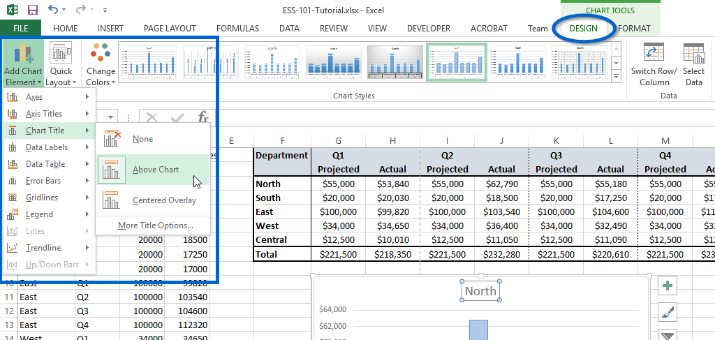
Add a chart title
Add axis titles
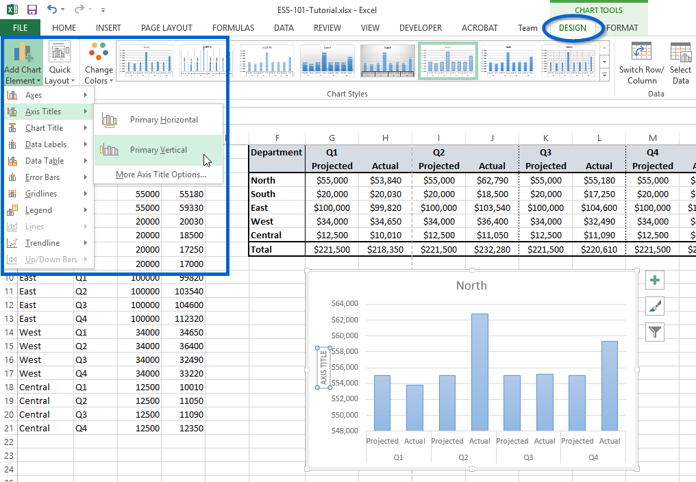 Add an axis title
Action Steps
Core Component:
6. Learn Keyboard Shortcuts to Improve Productivity
Keyboard shortcuts allow you to do most things in Excel with your keyboard instead of using your mouse. So why would you want to do this… Quite simply, to increase your speed and productivity. If you do a lot of data entry, having to take a hand off the keyboard and put it on your mouse then navigate to the ribbon, then make a selection etc, it is usually far simpler and much quicker to keep your hands on the keyboard and press a couple of additional keys.
Once you start using Excel more often, you soon learn some of the basic keyboard shortcuts that significantly improve your speed and productivity. Listed below are some shortcuts to get you started that once you have learnt them, you’ll wonder how you got along without them.
Keyboard Shortcuts |
||
| Shortcuts | Keys | To Achieve |
| Arrow keys |  |
Complete cell entry and move the cell cursor one cell in the direction of the arrow key pressed |
| Enter | Complete cell entry and move the cell cursor one row down | |
| Ctrl + C | Copy the cell(s) in the selected range | |
| Ctrl + V | Paste the cell(s) in the selected range | |
| Ctrl + X | Cut the cell(s) in the selected range | |
| Ctrl + Z | Undo the previous action | |
| Ctrl + N | Create a new workbook | |
| Ctrl + O | Open a workbook | |
| Ctrl + S | Save the workbook | |
| Ctrl + F4 | Close the workbook | |
| Esc | Cancel the current cell entry | |
| Ctrl + A | Select all cells in the selected range. Pressing Ctrl + A twice selects all cells in the entire worksheet. | |
If you are interested in learning some more keyboard shortcuts for Excel, the following article references shortcuts to improve productivity if you do a lot of data entry – 13 Keyboard Shortcuts for Data Entry, or see our 25 MUST have Keyboard Shortcut Cheatsheet.
Action Steps
What to do now…
This eCourse is designed to just scratch the surface of what Excel is able to do for you. It is by no means fully comprehensive but rather a guide to get you started.
By all means, if you have any questions or need clarification about anything within this tutorial, please leave a comment in the discussion area below.
Beyond the Kick-Start – Learning to “Kick” even further in Excel
After you have worked through this eCourse, we KNOW you will be wanting to know more.
The reasoning is simple:
- People with good Excel good Excel skills are always in demand;
- Your boss will love you because you accomplish tasks efficiently and effectively;
- Your clients will love you because you will be creating impressive reports and analysis;
- Your colleagues will envy you because your spreadsheets are easy to use and look great; and
- You’ll want to do more as you are starting to see how powerful a tool Excel can be and see endless opportunities to how you can apply it in your day to day activities.
To take your Excel learning experience to the next level, we suggest you START HERE.
