Excel formula basics every small to medium business owner should know.

One of the most powerful features of Excel is its ability to allow you, the user, to specify relationships between the information you have stored in your worksheets. Having the ability to be able to specify these relationships i.e. using formulas between your information, can significantly enhance and improve the usefulness of your spreadsheets.

Formulas allow you to turn your spreadsheets from static displays of data to useful tools being able to undertake calculations and show the results of the analysis. Turning jumbled data into meaningful information.

Excel Formulas

To begin, let us break down the structure of a formula in Excel so we can see how we can start to use them.

Thankfully all formulas in Excel are generally constructed the same way. They all start with an equals sign (=) followed by one or more elements. The equals sign simply tells Excel that we are storing a formula in this particular cell.

Each of the elements after the equals sign can be any or all of the following:

1. Constants
2. Operators
3. References
4. Functions

1. Constant

A constant is a value that is static and not the result of a calculation. For example, the numbers 1, 2, 3, 4, and 5 or even text like “ExcelSuperSite” are all examples of constants i.e. they do not change by themselves nor are they a result of a calculation.

A small but helpful tip – I usually stay away from using constants in formulas wherever possible as the result only changes after you modify the formula yourself. It is far better, from a spreadsheet design point of view, to use cell references in place of constants. This gets further discussed a little later.

2. Operators

Operators specify what type of operation (calculation) you want to perform on the elements in your formulas. There are four different types of operators that you can use:

a. Arithmetic
b. Comparison
c. Text
d. Reference

a. Arithmetic operators are used to perform basic mathematical operations such as addition, subtraction, or multiplication etc

Arithmetic Operator	Description	Example Formula	Formula Result
+	Addition (plus)	= 3 + 2	5
–	Subtraction (minus)	= 5 – 2	3
*	Multiplication (times)	= 3 * 2	6
/	Division	= 10 / 2	5
%	percent	= 20%	0.2
^	exponential	= 3 ^ 2	9

b. Comparison operators are used to compare two elements. The result of a comparison is a logical value either TRUE or FALSE.

Comparison Operator	Description	Example Formula	Formula Result
=	Equals	= 3 = 2	False
>	Greater than	= 5 > 2	True
<	Less than	= 3 < 2	False
>=	Greater than or equal to	= 10 >= 2	True
<=	Less than or equal to	= 10 <= 2	False
<>	Not equal to	= 3 <> 2	True

c. Text operators are used to join (concatenate) one or more pieces of text together.

Text Operator	Description	Example Formula	Formula Result
&	Concatenate (join)	= “Excel” & “Super” & “Site”	ExcelSuperSite

d. Reference operators are used to combine ranges of cells for calculations.

Reference Operator	Description	Example Formula
:	Range – references all cells between two references	=SUM(A1:A10)
,	Union – combines multiple range references	=SUM(A1:A10,C1:C10)
(space)	Intersection – references all cells common to the two references	=SUM(A10:D10 B5:B15)

Just like when you calculate a normal maths problem, Excel follows basic maths principles when it undertakes calculations. Excel starts from the left and works to the right obeying maths precedence rules

B O M D A S (Brackets – Order – Multiplication – Division – Addition – Subtraction).

If you combine more than one operator into a single formula, you can change the order of evaluation by using parentheses (brackets) to enclose the part of the formula to be calculated first.

As an example, the following formula results in 7 because Excel calculates multiplication before addition (obeying standard math precedence rules). The formula multiplies 2 by 3 and then adds 1 to the result. =1+2*3 = 7

However, if we add parentheses to change the calculation order we can end up with a result of 9 instead. Excel adds 1 to 2 and then multiplies this result by 3 to give a total of 9. =(1+2)*3 = 9

3. References

References in formulas tell Excel where to look for data or information to use in your formula.

Excel makes reference to cells in a worksheet by using the column letter and row number of the particular cell. As an example, cell reference C5 refers to the cell at the intersection of column C and row 5.

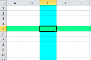
References allow you to use the value from one cell in multiple formulas throughout your worksheets. As discussed earlier, I highly recommend that you use this method to utilise constants in your formulas i.e. use a cell reference to the constant rather than the actual constant itself.

To try and explain this a little further, consider the following example:

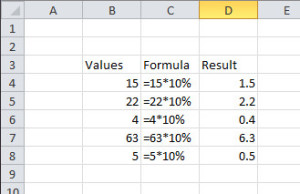
Let’s say we want to calculate 10% of the following list of numbers. Easy enough done. Simply enter a formula in each of the cells in column C as shown below.

Simple formula in Excel using Constants

Now that was easy enough, so why would you want to use references instead of constants in your formulas?

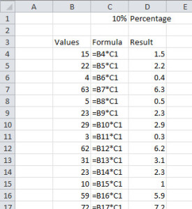
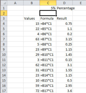
Consider the following extension to the above example. Instead of a list of 5 numbers to calculate 10% of, you now have a list of say 50 (or 5,000) numbers and to make things a little more interesting, you want to calculate a range of percentages, say 5%, 10%, and 15%.

This COULD be done exactly the same way as the above example but it will require a lot of manual editing of all your formulas to get it done. There is nothing wrong with working hard, but I also prefer to work smart as well.

So let’s start to get Excel to work for us rather than the other way round and us doing all the work.

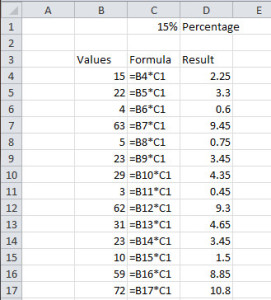
Before we modify the formulas in column C, let’s first enter the percentage constant into cell C1

[click cell C1 and then type “10%” {without quotes} then press enter]

In cell C4 type: = B4 * C1 then press enter

What this formula is saying is to take the value of whatever is in cell B4 and then multiply that by the value of whatever is in cell C1.

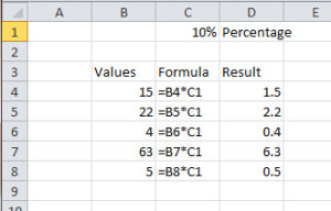
Now copy this formula down to all the cells in column C.

Formula using references in Excel

By entering the formula in this way, we can easily update the percentage constant in cell C1 to either 5% or 15%, as per our example, and we do not have to manually edit any of the formulas to get the results we are after. Similarly, all the values in column B could also be updated and we save ourselves a lot of work by having Excel do it all for us.

Image of Formula references in Excel - 10%

image of Formula references in Excel - 5%

Image of Formula references in Excel - 15%

References	Type
Reference to the cell in column C and row 1	C1
Reference to the range of cells in column C and rows 1 through 10	C1:C10
Reference to the range of cells in columns C to E and rows 1 through 10	C1:E10

4. Functions

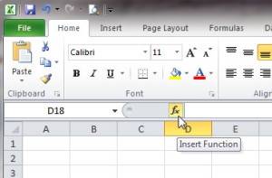
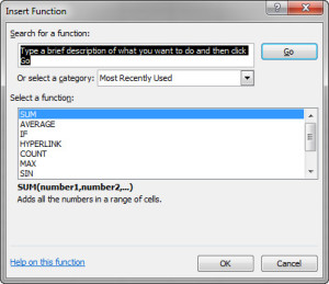
Functions are predefined formulas in Excel that are available for you to use. A full listing of functions available for you to use can be found by clicking any cell in Excel and then pressing SHIFT & F3 (together) or by clicking the Insert Function button beside the Formula Bar.

Some of the more common functions include SUM, COUNT, AVERAGE, MIN, MAX etc. I am not going to go into these functions in this post but will follow up with posts about each of them, so we can look at each in a lot more detail.

Image of How to insert a function in Excel

Help support ExcelSuperSite – T-Shirts and Merchandise

Do you like this template and would like to help support us at ExcelSuperSite to continue to share great templates and content such as this – why not take a look at some of the t-shirts and merchandise we have on offer – click any of the images below to visit our store.

Please note – our T-shirts and merchandise are hosted on an external “Print on Demand” website Redbubble/ExcelSuperSite so when you click an image below you will be automatically taken to our store on that site.