HOW TO SHADE ALTERNATE ROWS WITH CONDITIONAL FORMATTING
Here at ExcelSuperSite, we regularly work with large sets of data. One quick and simple “trick” we use ALL the time is to shade every alternate row in our data. This makes our data easier to read and gives it that professional “look ‘n’ feel”.
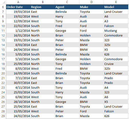
Take a look at the example shown below, by itself, it is a very visually unattractive spreadsheet. It is full of lots of data and is very hard to read.
The readability of this data can be significantly enhanced by shading every alternate row using Conditional Formatting.

Simply put, Conditional Formatting automatically applies different formatting styles (colours, background shading etc) to your data based. The styles applied are based on the criteria you set.
For this particular tip, we use Excel row numbers to work out which row to shade (or not).
Excel Tip – How to shade alternate rows with Conditional Formatting
Now on to the tip:
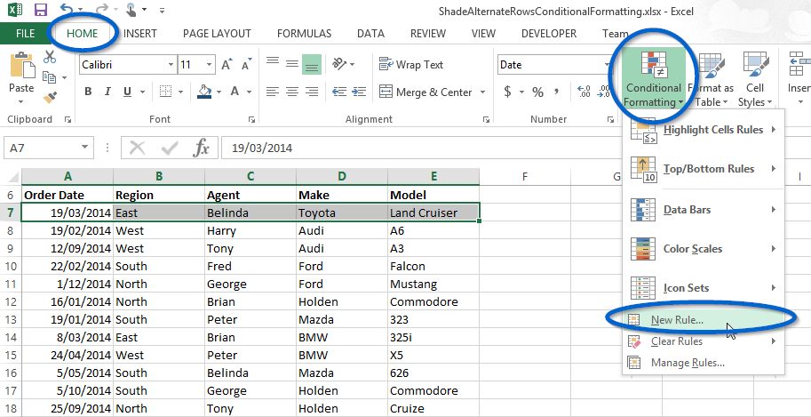
Step 1 Select the first row of your data (cells A7 to E7 in my example below)
Step 2 On the Home tab, select Conditional Formatting, then click New Rule…
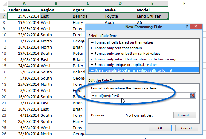
Step 3 In the New Formatting Rule dialogue box, select the Use a formula to determine which cells to format
Step 4 In the Format values where this formula is true: box type the following formula:
=mod(row(),2)=0
The ROW() function brings back the row number in which the formula appears. For the highlighted row in the image shown below, row() would return the value 7.
The MOD function returns the remainder of a number after it is divided by a divisor. Hence when we use row numbers and a divisor of 2, the remainder of every 2nd sum will equal 0. That is, the MOD (or remainder) of row 1 divided by 2 equals 0.5, the MOD (or remainder) of row 2 divided by 2 equals 0, MOD row 3 = 0.5, MOD row 4 = 0 and so on.
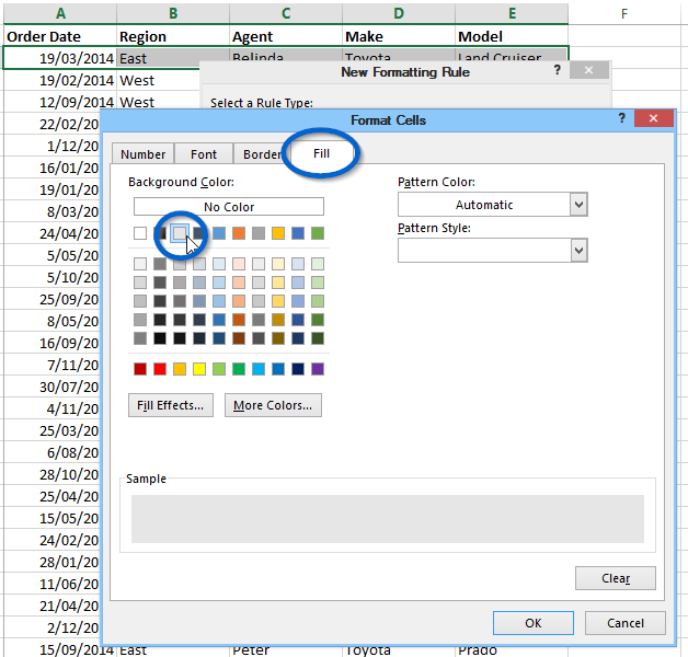
Step 5 Next, click the Format button and select a pale background fill. The colour that you select will become the colour that is applied to the background of every alternate row.
Step 6 Click the OK button and OK again to apply the Conditional Formatting to your first row of data.
Step 7 Conditional Formatting is now set up for your first row of data. This formatting needs to be copied to your remaining rows of data.
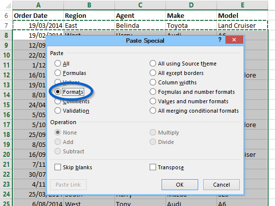
Step 8 In our example, select cells A7 through to E7 and click the Copy button (or CTRL+C).
Step 9 Select the remaining rows of data and use Paste Special, Formats to paste the Conditional Formatting to this remaining data.
Your data will now have the Conditional Formatting rules applied to it. Every alternate row should now be automatically shaded making it far more readable.
Nb: We “cheated” a little in the image above. The title row was also changed to have a dark background and white font, to make it stand out from the rest of the data.
But wait, That’s not all…
Assuming you now want to shade every third row of data in your information. Simply modify the “=mod(row(),2)=0” formula by changing the 2 to a 3 (i.e. “=mod(row(),3)=0”). Or if you want every fourth row of data shaded, change the 2 to a 4 (i.e. “=mod(row(),4)=0”).
Ok that’s it for this tip. As always should you have any questions or queries about any information we have provided, let us know.
Till next time.
Please Share
If you liked this or know someone who could use it, please click the buttons below to share it with your friends on LinkedIn, Google+, Facebook and Twitter.
Download
You can download a PDF transcript of this tip by clicking the following link – How to shade alternate rows in Excel using Conditional Formatting.
You can also download a copy of the spreadsheet I used in this article so you can explore this tip further – How to shade alternate rows in Excel using Conditional Formatting spreadsheet.
Video
Lastly, if you prefer you can watch an explanation of this tip in the video below.